We have a company that is concerned with its attrition. Employer turnover is disruptive and expensive, SHRM estimates that replacing an employee can cost anywhere from 50% to 200% of the role’s annual salary. Understanding who is likely to leave, and why, can help us take proactive steps to reduce talent costs, retain talent, and preserve institutional knowledge. This company in particular is trying to get ahead of the game by asking the question, what drives attrition?
Summarized Key Insights
Respect for Time
Employees who worked Overtime had over 300% higher odds of leaving compared to those who didn’t work overtime, far and away the strongest predictor of attrition.
Employees who frequently traveled for work also had high attrition rate, 90% higher odds of leaving compared to those who didn’t travel.
Risky Roles: Sales & Labs
Two job roles had notable turnover–Sales Representatives and Laboratory Technicians.
Who Stays? Involved, Happy Workers
No surprise to see that, but what is important is to know by how much–each point higher a worker scored on Job Involvement, Environment Satisfaction, and Job Satisfaction reduced their odds of leaving by nearly 20%-30%
Recommendations
Adapt schedules to reduce Overtime needs. Review budget optimization by exploring whether increasing headcount to reduce overtime may be a cheaper option than dealing with the high turnover caused by stretching fewer workers into overtime.
For Example: If baseline attrition is 10%, shifting 100 employees out of Overtime could avoid approximately 22 exits, saving about $677k (assuming $30k per replacement cost)
Prioritize improving Job Involvement (perhaps: enhance role clarity, autonomy), Environment Satisfaction (perhaps: modernizing workspaces, hybrid/remote policies), and Job Satisfaction (perhaps: emphasizing recognition, fair workload) to retain more workers.
For Example: If baseline attrition is 10%, getting all employees to score on average 1 point higher on Job Involvement could avoid approximately 41 exits, saving about $1.2 million (assuming $30k replacement cost)
Especially look at Sales Representative and Laboratory Technicians to examine their pain points.
Fun Facts
Age and Total Working Years had near zero effect on attrition–no evidence for any effect in either direction. This company seems to buck typical industry trends (e.g., where total working years tends to on-average increase attrition risk).
Method & Data
Data
The data come from IBM’s fictional HR Employee Attrition and Performance data, available for download via Kaggle. The dataset includes approximately 1500 employees with personal features (e.g. years working, age, gender), role characteristics (e.g. business travel frequency, department, monthly income), and engagement details (e.g. job satisfaction, rating of work life balance).
Method
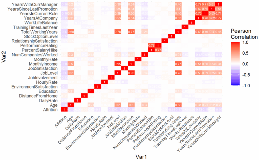
I moved the dataset into RStudio for quality checks and analysis. Data exploration suggested no significant missingness or necessary corrections for analyses. Exploratory visualizations showed moderate to weak associations with attrition (e.g. see correlation plot below). This suggests a lack of “obvious” predictors of attrition. Furthermore, the inter-correlations between other predictors (e.g. the top right block of the correlation plot) suggest it will be important to get more precise about the unique explanatory power of each predictor on attrition. Doing that requires a linear model, but with so many predictors we risk overfitting to our data and over-complicating our model. I.e., I want to select which features are actually ‘doing something’ out of this huge bag of variables, but if I use all of them I risk getting too tied to this specific dataset–enter LASSO Logistic Regression.
Note: Attrition (bottom left corner column/row) has weak, negative correlations with most continuous variables.
A logistic regression is the standard generalized linear model framework for binary outcome variables. LASSO is a regularization method for linear models that reduces overfitting from using a high number of features by shrinking the coefficients of statistically unimportant variables to zero. The model thus only displays features that have “survived” the LASSO penalty, identifying only the most relevant features to interpret. I ran a LASSO logistic regression predicting attrition (yes/no) against all data features.
Technical Findings
Results
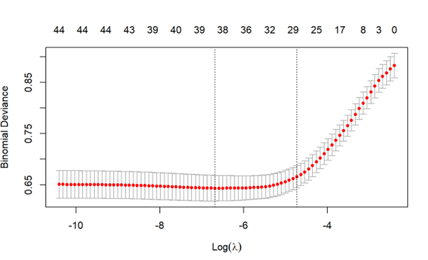
Model Evaluation
Here is our model evaluation plot of binomial deviance, showing the minimum deviance model (far left dotted vertical line) and 1SE minimum deviance model (right dotted vertical line). The minimal model reduces error by the most but also is most liable to be overfitted to our data (smallest penalty -> allows the most predictors). Meanwhile, the 1SE model has near similar error reduction but is a simpler model and in this case is not notably “worse” of a model compared to the “best” minimal model (note the near horizontal performance from around x = -5 onward, even with further lambda penalty reductions). To maximize simplicity for reduced deviance, I chose the 1SE model.
For more about this LASSO plot diagnostic, see here.
A LASSO logistic regression is often evaluated by how much deviance, or “error”, we reduce based on how many predictors we have in our model doing ‘real statistical/explanatory work.’ The “LASSO” part of this regression adds penalties for how much ‘stuff’ we threw in our model–if we have a huge penalty, making all the predictors we threw in zero, we’ve basically made an intercept-only model. This intercept-only is the far right of the figure; this shows how much deviance (‘error’) we’d have if we just applied the average attrition rate to everyone–i.e. “I don’t know or care about any details of this person; our attrition rate is X%? Ok, it’s not perfect, but I’ll just say everyone has those odds to leave.” As we lessen the penalty, moving left across the graph, we allow more and more predictors to play a role in the model. That means our error will go down until we’ve done as much ‘explaining’ as possible with these given variables. The question is then–at what point have we minimized the error? And then, did we overfit our data (i.e. minimize it too much)? That is where one must decide the appropriate penalty (Lambda hyperparameter) that A) has much improved the deviance from the far-right intercept-only model, B) minimizes the deviance (‘error’), and C) is as parsimonious as possible; it’s the goldilocks situation of wanting a high enough penalty (as far right side of X-axis as possible) that has removed as many ‘extra’ predictors as possible while also reducing as much deviance as possible (as far down on Y-axis as possible) which typically requires more and more predictors.
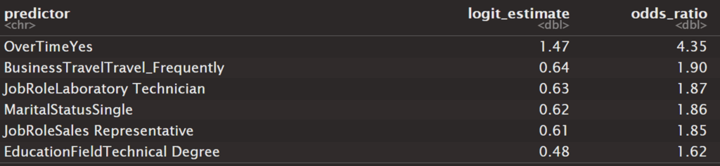
Top Coefficients
What do those numbers mean?
Each coefficient is directly from the logistic regression (in “logit” units, which are unhelpfully confusing for most interpretation purposes). Converted to odds ratio, they now reflect the change in odds for each feature–numbers above 1 make attrition more likely, numbers below make attrition less likely. For example: Overtime has an odds_ratio of ~4, thus a ~4x higher odds than No Overtime employees. Remember, odds of 1 mean no difference either way (it’s short for odds 1:1). Meanwhile, employees in R&D (not shown) have an odds_ratio of .63 meaning the odds of an employee from R&D are only .63x that of other employees, i.e. they have lower odds (specifically, reference group here is HR due to alphabetical dummy coding).
Limitations
These data are not necessarily causative: Correlation does not equal causation, as always. Attrition data has slightly more causative logic than other cross-sectional data analysis (attrition has temporal precedence, a key component of determining causality, baked in), however one should not overgeneralize without deeper understanding of the business and it’s field.
Odds ratios are relative: Odds ratios quantify relative likelihood, thus depend on the base probability of something. I.e. Overtime may pose a 4x odds risk of attrition, but if the attrition risk is very low then the actual change may remain small.
Data may miss un-tracked, macro features that influence attrition for the company (e.g. macro-signals such as economic outlook or job market conditions) or limited internal scope (e.g. does not include other potentially important predictors like manager quality, team culture) or other company developments (e.g. M&As, recent layoffs etc.).
Demonstration Dataset: These data come from an IBM simulated dataset and thus may not generalize to real-world dynamics.
You probably know someone with anxiety or depression; a friend, a loved one, a colleague, maybe even yourself. And no wonder, the world often seems all too enthusiastic to doll out stuff to get anxious Read more…
Goal Let’s pretend… The State of Hawaii is looking to update their aging infrastructure, particularly to help reduce their environmental impact. A potential solution is replacing cesspool systems in favor of sewage systems that are Read more…